A robot can finish its motion quickly and still spend most of the cycle waiting. A clamp has not confirmed. A process timer is running. The next station is occupied. Increasing robot speed will not remove those delays.
A useful cycle time study starts with the operating sequence and its dependencies. It asks what sets the interval between completed parts, then checks whether the selected equipment and controls can support that interval.
Define the number you are trying to meet
Distinguish robot motion time, a station cycle, the interval between finished parts, and the time one part spends in the system. These can be different in a cell with parallel operations or buffers. State the product mix and whether the target describes nominal operation or sustained output over a specified period.
Customer demand also matters. If 420 net available minutes must support 700 good parts, the implied demand interval is 36 seconds per good part. This illustrative calculation is not a machine capability claim. It establishes a planning target before accounting for the actual process constraints and the agreed treatment of losses.
Map dependencies before summing durations
| Step | Time | Dependency |
|---|---|---|
| Load | 4 s | Station available |
| Clamp and confirm | 2 s | Part located |
| Process | 18 s | Clamp confirmed |
| Release | 1 s | Process complete |
| Unload | 4 s | Release confirmed |
The nominal total is 29 seconds under these assumptions. Cutting load time from four seconds to three saves one second, not a proportionate share of the whole cycle. If loading can legitimately overlap another operation in a different layout, the model must represent that concurrency rather than subtracting time informally.
Identify shared resources as well: one robot serving two fixtures, a common inspection station, or a transfer path that cannot accept two parts at once. These constraints can move the bottleneck away from the longest individual operation.
Verify the assumptions behind each component time
For motion, use the selected mechanism, travel, acceleration assumptions, payload, and path. For pneumatic devices, review the relevant operating conditions and confirmation behavior. For processing equipment, distinguish a proven dwell requirement from an estimate. Include the control and interface delays that are material to the sequence.
Label each timing input as measured, supplied by a manufacturer, calculated, simulated, or assumed. An attractive animation does not establish the accuracy of its timing inputs. ABB identifies reach, cycle-time, layout, and flow evaluation as uses of digital simulation in its machine-tending guidance; the project model still needs the correct application data.
Test variation rather than hiding it in a margin
Run agreed scenarios for a slower process step, an occupied downstream station, different product variants, and realistic operator interactions. Where variability matters, a nominal deterministic sequence alone may not answer the throughput question.
Show the sensitivity explicitly. If a process dwell grows by three seconds, does the output interval also grow by three seconds, or does a buffer temporarily absorb it? If a proposed faster robot barely changes output, the investment decision should reflect that result. Do not apply a generic efficiency percentage without explaining its source and what it represents.
Finish with a decision and a verification plan
The study should identify the bottleneck, achievable timing under the stated assumptions, differences between alternatives, and inputs that still require physical confirmation. Record whether the proposal is to change a component, adjust the sequence, add parallel capacity, or revise the target.
Keep the predicted result separate from an acceptance guarantee. The final production commitment needs agreed test conditions, representative parts, and a method of measuring output. That makes the simulation useful both during design and when planning the eventual acceptance test.